Data

If you want to skip the background for now, go and download the data directly.

This year’s contest deals with the simulation of activity within the human brain, especially the changes within its network structure. Current understanding suggests, that a large amount of connections between neurons via synapses is constantly changing, leading to alteration of brain functionality. This includes positive effects such as the creation of memories [ 1 ] or negative ones such as limitations caused by accidents or illnesses [ 2 ] .
To understand these effects on a neuronal level, scientists hope to artificially recreate networks that work similarly to the human brain with the help of simulation models. The data provided in this contest is based on clinical measurements of actual human brains as well as the Model of Structural Plasticity by Butz & Van Ooyen [ 2 ] which can be coarsely summarized as follows:

The brain is modeled by a network of neurons. Each neuron is represented by a node with a number of properties such as location, calcium concentration, and target calcium concentration. It can further carry axonal (“plugs”) and dendritic (“sockets”) elements. If two neurons are spatially close and exhibit unused complementary elements, they have a probability to form a synapse, which is represented by a connection in the network through which electric energy can be passed from one neuron to another if it “fires” based on external input and the Izhikevich model [ 3 ] . When a neuron fires, its calcium level increases only to decrease again over time. In this model, neurons aim to reach a certain target calcium concentration based on their current calcium level. To achieve this, it either seeks to increase or decrease the level of incoming electrical activity resulting in the addition or removal of elements, which, in turn, leads to the formation, rewiring, or deletion of synapses.
Thus, in each simulation step, each neuron calculates its energy income and calcium level based on this model, followed by the addition or deletion of elements, leading to changes in the network structure. This can be repeated until the system has reached a stable configuration or stopped on demand.

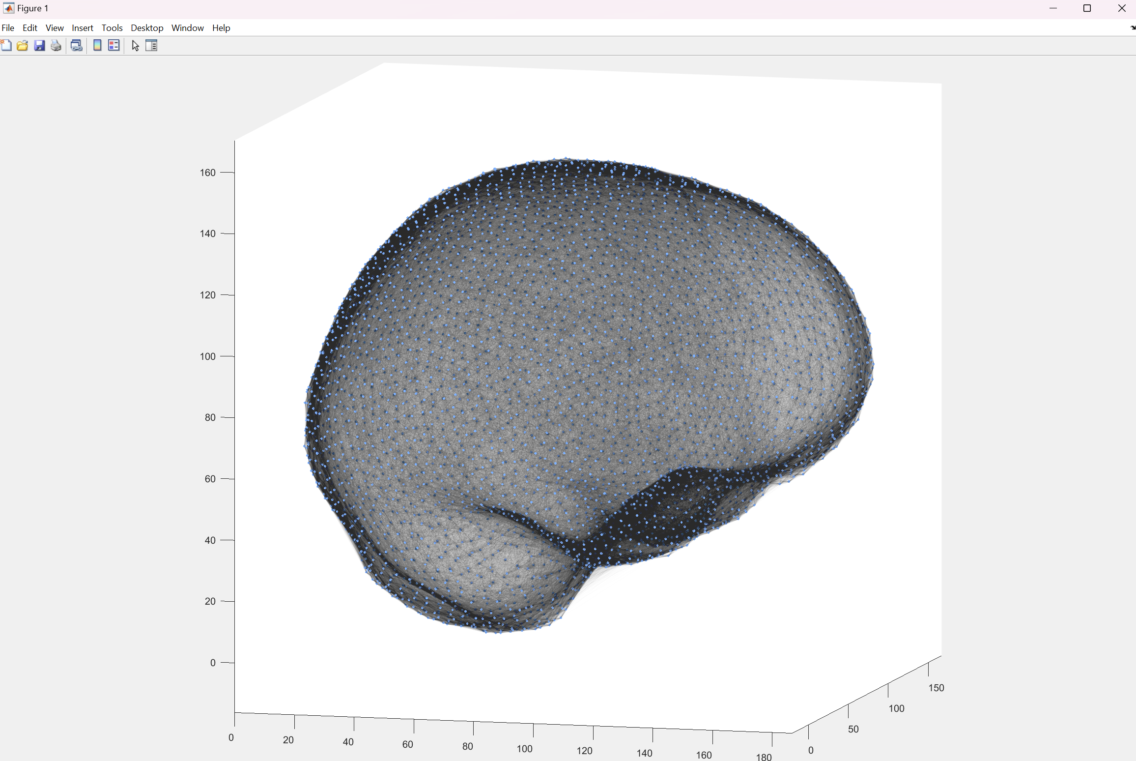
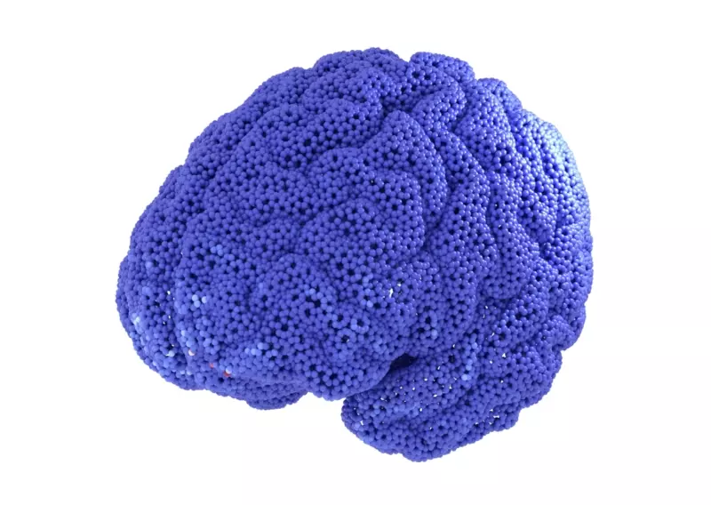
The following animation shows a simple visualization of a similar dataset: The neurons are represented as spheres at the appropriate locations and colored by their current calcium level.

Animated Brain

On the front page you can also see a visualization containing line renderings of ingoing connections (synapses) of the same dataset.

Visualization can help to understand these processes (see, e.g., [ 4 ] ). Therefore, the goal of this contest is to enable domain scientists as well as simulation scientists to better evaluate their models, compare, and explore the simulation results. Based on this, we have provided a list of visualization tasks for this contest.


Data Description

Summary

This data contains:

  • ~50 GB data
  • 4 simulation ensemble members
  • Each members consists of 50 000 neurons
  • Each node collects information about 12 parameters
  • The simulation is run for 1,000,000 simulations steps
  • Every 100th iteration step is sampled per node

Please find more details in the readme.md.

In-Detail Description

Four simulations have been run based on neuron locations given by the same underlying human brain data (MEG 146129) provided within the human connectome database [ 6 ] and extended by additional neurons close to existing ones. In the future, we plan on using more accurate models but these are not yet open for free use. Technical details on the simulation process can be found in [ 7 ] and [ 8 ] . Each simulation produces several text files sorted in their corresponding folder:

Simulation Conditions: Folder Name
1 0-calcium level at the start and equal target calcium level for all neurons, no existing connections no-network
2 Lesion Simulation: Take the connection result of 1 and simulate with 10% neurons inactive (dead). disable
3 Learning Simulation: Take the connection result of 1 and simulate learning (electric stimulation) of a specific area stimulus
4 Take the connection result of 1 and use different target calcium levels for neurons calcium

Some of the simulations have additional files, e.g., calcium_targets.txt,disable.txt, and stimulus.txt that include simulation specific information.

As the simulation can be efficiently run on a cluster of computing nodes, MPI information is included within the files and names by a leading MPI Rank ID.

Each folder has the same setup explained in the following:

Network Layout

The base for the simulation is a neuronal network represented by point neurons. Each neuron has a Neuron ID that is unique to its MPI Rank ID. The combination of both is then used throughout the simulation and data.

The 3D-position of each neuron can be found in positions/rank_0_positions.txt.
These are fixed and do not change. This file further contains labels explaining which part of the brain the neuron belongs to. Note: These areas are set manually and are not based on medical accurate regions within the human brain.

Ingoing as well as outgoing connections between nodes are sampled at different simulation steps and written in network/<MPI_RANK_ID>_step_<STEP>_in_network.txt and network/<MPI_RANK_ID>_step_<STEP>_out_network.txt respectively.

Per Node Information

The information about individual nodes is saved to *.csv files within monitors.zip.
Their naming convention is as follows: <MPI_RANK_ID>_<NEURON_ID - 1>.csv.
Each row within the file contains the per-node information at a sampled simulation step.

The following parameters are listed:

Variable Description
Step Sampled simulation step
Fired Boolean: Did the neuron fire within the last sample step
Fired Fraction In Percent: Number of firings since the last sampling
x Electric Activity
Secondary Variable Inhibition variable used for the firing model of Izhikevich
Calcium Current calcium level
Target Calcium Target calcium level
Synaptic Input Input electrical activity
Background Activity Background noise electric activity input
Grown Axons Number of currently grown axonal boutons
Connected Axons Number of current outgoing connections
Grown Excitatory Dendrites Number of currently grown dendrite spines for excitatory connections
Connected Excitatory Dendrites Number of incoming excitatory connections
Simulation Information

Each simulation run also saves some statistics:

File Name Description
neurons_overview.txt Statistical summary sampled simulation steps
plasticity_changes.txt Summary of creation and deletions of connections
stdcout.txt Program output
timers.txt Timings
Matlab example for visualizing nodes and connections

This is a small hacked example of how to read node positions, incoming connections, and calcium value and plot the network in Matlab.

The code example below should produce the following outcome:

Matlab Plot
% Assuming the correct file locations have been set
%%% First we read in nodes and their locations
fileID = fopen(positionfilelocation,'r');

% Read number of nodes:
numOfNodes = fscanf(fileID,'# %d');
fgetl(fileID);

% Read min max values:
minMaxXYZ = fscanf(fileID,'%*s %*s %*s %f',[3,2]);
fgetl(fileID);
fgetl(fileID);

% Read positions, labels and type
data = textscan(fileID,'%*f %f %f %f %s');
fclose(fileID);

% Data containters
positions = [data{1} data{2} data{3}];
labels = [data{4}];

%%% Now read the incoming connections:
fileID = fopen(connectionInfilelocation,'r');
fgetl(fileID);fgetl(fileID);fgetl(fileID);fgetl(fileID);fgetl(fileID);
inconnect = textscan(fileID,'%f %f %f %f %f');
fclose(fileID);

%%% Read Calcium values:
fileID = fopen(calciumfilelocation,'r');
str = fgetl(fileID);
iterations = 0;
calcium = zeros(1,numOfNodes);

i = 1;
while(str ~= -1)
    linedata = strsplit(str,';');
    iterations(i) = sscanf(linedata{1},'#%d');
    calcium(i,:) = str2double(linedata(2:end));
    i = i+1;
    str = fgetl(fileID);
end
fclose(fileID);

%%% Plot Nodes and incoming connections
f = figure
hold on
axis vis3d
% optional: set(f,'renderer','opengl');
view(60,8)

% plot ingoing connections:
xx = [];
for i=1:size(inconnect{1},1)
    startnodeid = inconnect{2}(i);
    endnodeid = inconnect{4}(i);
    line = [positions(startnodeid,:);positions(endnodeid,:)];

    xx(((i-1)*3)+1:((i-1)*3)+3,:) = [[line(:,1);NaN],[line(:,2);NaN],[line(:,3);NaN]];
end
h = plot3(xx(:,1),xx(:,2),xx(:,3),'-k');
h.Color(4)= 0.01;

% plot neuron locations
plot3(positions(:,1),positions(:,2),positions(:,3),'.','Color', "#80B3FF")

Be warned: due to the number of nodes, plotting might be very slow on some machines.


Download Data

The data has been published on zenodo, using the following link:

https://zenodo.org/records/10519411

If you use this data set in your publications, please acknowledge the following:

Dataset:
Gerrits, T., Czappa, F., Banesh, D., & Wolf, F. (2022). IEEE SciVis Contest 2023 - Dataset of Neuronal Network Simulations of the Human Brain (1.0) Zenodo. Link Zenodo page

Neuron positions based on:
Marcus DS, Harwell J, Olsen T, Hodge M, Glasser MF, Prior F, Jenkinson M, Laumann T, Curtiss SW, and Van Essen DC. (2011). Informatics and data mining: Tools and strategies for the Human Connectome Project. Frontiers in Neuroinformatics 5:4.

Simulation based on:
Rinke, Sebastian and Butz-Ostendorf, Markus and Hermanns, Marc-André and Naveau, Mikael and Wolf, Felix. (2018): A scalable algorithm for simulating the structural plasticity of the brain [ 8 ].


References and Acknowledgments

The contest is organized by the Crosssectional Group Visualization and the Crosssectional Group Parallelism and Performance within the National High Performance Computing Center for Computational Engineering Science (NHR4CES [ 5 ] ).

[1] Gallinaro, Júlia V. and Gašparović, Nebojša and Rotter, Stefan (2022): Homeostatic control of synaptic rewiring in recurrent networks induces the formation of stable memory engrams - Available here
[2] Butz, Markus and van Ooyen, Arjen (2013): A simple rule for dendritic spine and axonal bouton formation can account for cortical reorganization after focal retinal lesions - Available here
[3] Izhikevich, Eugene M. (2003): Simple model of spiking neurons - Available here
[4] Nowke, Christian and Diaz-Pier, Sandra and Weyers, Benjamin and Hentschel, Bernd and Morrison, Abigail and Kuhlen, Torsten W. and Peyser, Alexander (2018): Toward rigorous parameterization of underconstrained neural network models through interactive visualization and steering of connectivity generation Available here
[5] National High Performance Computing Center for Computational Engineering Science (NHR4CES) - Website
[6] https://db.humanconnectome.org/
[7] Czappa, Fabian and Geiß, Alexander and Wolf, Felix (2022): Simulating Structural Plasticity of the Brain more Scalable than Expected - Available here [8] Rinke, Sebastian and Butz-Ostendorf, Markus and Hermanns, Marc-André and Naveau, Mikael and Wolf, Felix. (2018): A scalable algorithm for simulating the structural plasticity of the brain - Available here